In 1940, Nicholas Kaldor published in the Economic Journal a famous article presenting a new model of the trade cycle.1 Its main mechanism relied on the discrepancies between ex-ante saving and investment to explain the changes in the level of activity, and it introduced two important variations to this idea: (i), saving and investments were themselves functions of the level of activity, and (ii) the stock of capital was slowly varying. This make of his model a medium-run model of economic fluctuations, where oscillations arise endogeneously because of the non-linear relations between the two curves of investment and savings.
While Kaldor did not construct a fully worked out model, he suggested a graphical interpretation that was very clear and ensured his ideas had a great influence. Several economists sought to translate them into a formal model, and one of the most successful of such interpretations was given by Chang and Smyth in an article published in the Review of Economic Studies in 1971.2 In this post, I go back on the original mechanism of Kaldor’s model and compare it with the model formulated by Chang and Smyth. I then build an interactive version of the model that tries to encapsulate their ideas, with an estimation of the nonlinearity in the savings function.
The mechanism of fluctuations in Kaldor’s original model
While there had already been many influential models of the trade cycle, Kaldor thought that they lacked some explanatory powers, in particular because they postulated either too much or too little stability, in particular because they were based on mostly linear relationships:3
“Since thus neither of these two assumptions can be justified, we are left with the conclusion that the I(x) and S(x) functions cannot both be linear, at any rate over the entire range. And, in fact, on closer examination, there are good reasons for supposing that neither of them is linear.” (Kaldor, 1940: 81)
The curved form of the investment and saving functions were based on first principles, for instance the fact that high incomes meant not only that a higher amount was saved, but a higher proportion of total income was saved. At the opposite end, under a certain level of income, nothing was saved. Inversely, for investment, the nonlinearities can be thought of as maximum and minimum levels of investments determined by general technical and institutional conditions (such as the current stock of capital). The form of the curves ensured that they met at three points corresponding to three different levels of income, where the highest and lowest equilibrium are stable, and the middle one unstable.4 The economy can thus settle either at a high level of activity (\(X\)) or a low level, which can be seen in the “Stage I” picture of the following figure, taken from Kaldor’s article.
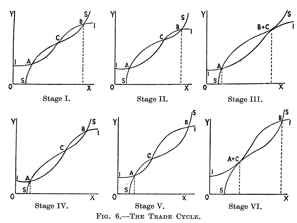
In Kaldor’s model, fluctuations actually happen between the high and the low equilibria, because these equilibria are only stable in the short run: “as activity continues at either one of these levels, forces gradually accumulate which sooner or later will render that particular position unstable” (ibid.: 83).
To explain why the equilibria become unstable, it is necessary to introduce the medium-run evolution of both investment and saving curves when the economy is at the high or at the low equilibria. At the high equilibrium, the stock of capital is gradually increasing, and so is the total amount of consumption goods produced. The level of savings is increasing and the S curve shifts upward, while investment is depressed and shifted down by the tightening of profit opportunities, due to the accumulation of capital. At some point the economy will reach stage three where there are only two equilibria left, and the high equilibrium is unstable downward: savings become higher than investment and the level of activity will decrease until they are equal again - at the low equilibrium A.
Once the economy reaches the low level equilibrium, the inverse movement will happen: the level of savings decrease and S shifts downward, while investment opportunities arise from the decumulation of capital. At some point there is two equilibria again, but this time the low equilibrium is upward unstable and the high equilibrium becomes a stable attractor, and the cycle between the two level of activity will endlessly repeat - unless something is done to stop it, that is, to prevent the high equilibrium from becoming unstable.
Kaldor thus ends his exploration of this idea with some considerations on the amplitude and duration of those cycles, and the implications for economic policy. The most important consequence is that it is necessary to ensure the level of investment is high enough to avoid that the high equilibrium becomes unstable; there is obviously a strong role the government can play to keep investment opportunities high, and to intervene directly on this schedule when the private sector is letting it shift down.
Chang and Smyth’s model: capital and income dynamics
Chang and Smyth proposed a dynamic formalisation of Kaldor’s model, that clarified important points that were missed by Kaldor, in particular the fact that the initial conditions and the parameter values were crucial for a limit cycle to arise and to avoid a monotonous convergence to a stationary-state equilibrium.
The model is based on a system of nonlinear differential equations with two variables, capital and income. Investment and savings depend on the level of income (positively) and the stock of capital (negatively). The dynamic of income depends on the difference between investment and savings, as in Kaldor’s model, and on a speed of adjustment \(\alpha\):
\[\frac{dY}{dt} = \alpha[I(Y,K) - S(Y,K)]\]For the dynamics of capital, several interpretations have been proposed in the litterature, as underlined by Chang and Smyth (1971: 39, n.2). They retain the simplest possible evolution, where the accumulation of capital is only a function of net investment:
\[\frac{dK}{dt} = I(Y,K)\]The authors then proceed to show that Kaldor’s conditions for the presence of limit cycles are not necessary nor sufficient in the general case by using the Poincaré Bendixson theorem. It is however regrettable that they do not give a numerical example for their model, and limit themselves to a hand-drawn figure of the locuses of points where investment equals savings and where net investment is null (that is, the set of points in the Y-K plane where income and capital are respectively stationary). Their diagram is reproduced below.
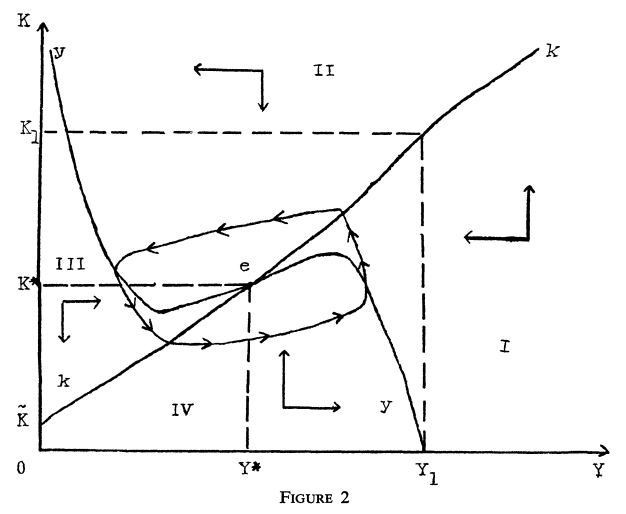
It is apparent from their model that there is one point of stationary equilibrium, \(e\), where both capital and income are stationary. The last section of their paper proves that Kaldor’s model will usually converge to this point, although there exists a set of points who give rise to the type of limit cycle represented in the picture. There can be several limit cycles, in which case the initial conditions will determined the ultimate cyclical behaviour of the economy.
Contrary to Kaldor, they do not seem to assume that the dynamics of the capital stock depends on its depreciation, although this was a crucial hypothesis in Kaldor’s article, who argued that “at the level of investment corresponding to A investment is not sufficient to cover replacement, so that net investment in industrial plant and equipment is negative” (Kaldor, 1940: 84). This “decumulation” of capital had the effect to increase investment opportunities and to decrease savings “in so far as it causes real income per unit of activity to fall” (ibid.: 85).
This makes the solution of their system quite strange in fact because if one looks at the two equations above (which are directly taken from their theorem p.41), we can readily see that income and capital will be stationary only when investment and savings are both zero. I suppose one could argue that this corresponds to a situation where we only take into account net investment and savings but I do not see how to reconciliate this with the picture drawn by Kaldor where investment and savings are always positive. Thus we slightly change their equation for the evolution of the capital stock to show the effect of capital depreciation, which allows us to obtain stationary points for positive values of investment and savings:
\[\frac{dK}{dt} = I(Y,K) - \delta K\]Where \(\delta\) is a measure of the rate of depreciation of the stock of capital. To understand this behavior better, and because this blog is more oriented toward numerical computation, I skip their proof and present in the last section of this post a specification of the forms of I and S that give rise to a limit cycle for different values of parameters.
Numerical specification of Chang and Smyth’s model
In this last part, I search for a model of the investment and saving functions that make sense economically, and that exhibit the required properties giving rise to limit cycles. To simplify the task, I use data from the St. Louis Federal Reserve5 and use simple regression methods to find statistically significant relations between income, capital, investment and savings.6
While both Kaldor (1940: 82) and Chang and Smyth (1971: 38) underline that it is not necessary for both the investment and saving curves to be nonlinear, I found that it was easiest to find the right locus in the K-Y plane with nonlinear forms for both. The model retained for the investment function is:
\[I(Y,K) = I_y \cdot Y + I_k \cdot K + I_{ky} \cdot Y \cdot K + \bar{I}\]Where \(I_y\), \(I_k\), \(I_{ky}\) and \(\bar{I}\) are all parameters estimated with a simple least square regression. The coefficients are summarised in the following table:
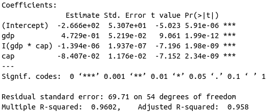
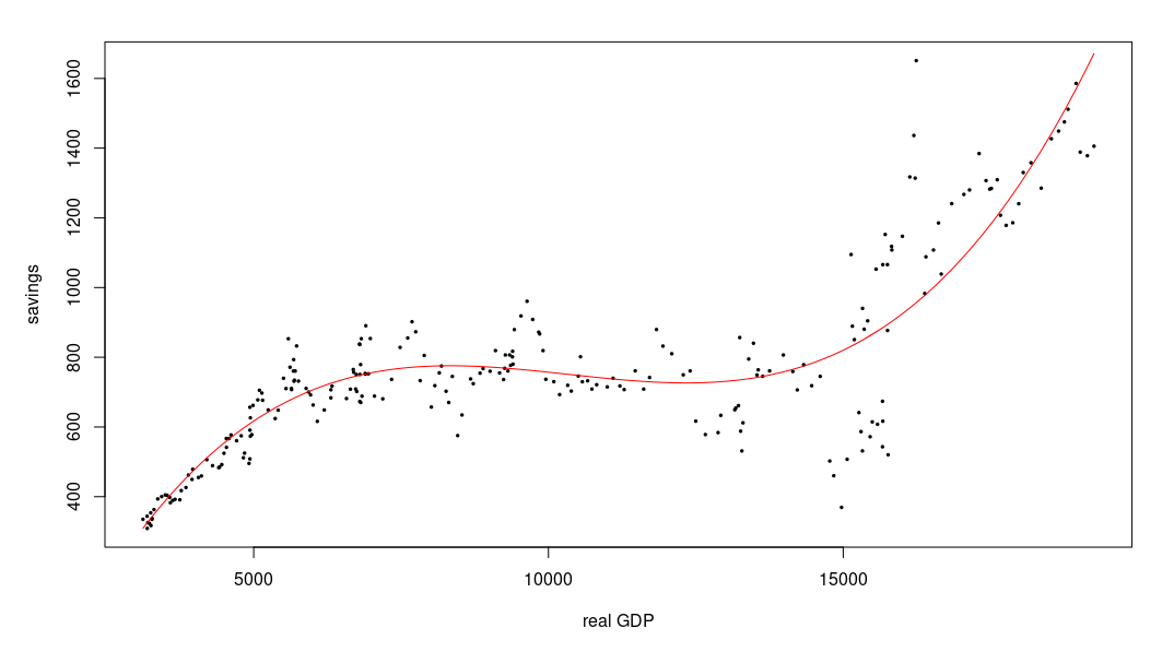
A nonlinear form of the savings curve can be found in an article by Klein and Preston,7 who estimate a logistic relation between consumption and income based on UK data, to construct a nonlinear limit cycle of Kaldor’s type. At first I just used a cubic model that showed an undeniable improvement over simple linear or quadratic relations while a quartic model did not bring anything to the fitting. The cubic model also exhibits the required properties (see the figure below).
The final model also includes a cross term between income and capital that gave rise to a better behaved locus of stationarity in the phase plane:
\[S(Y,K) = S_{y} \cdot Y + S_{y2} \cdot Y^2 + S_{y3} \cdot Y^3 + S_{yk} \cdot Y \cdot K + \bar{S}\]We obtain the parameters summarised in the following table for this model.
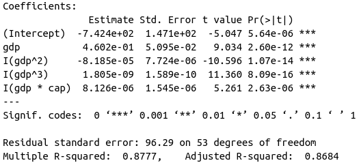
The fact that we have a negative intercept is in line with the idea that under a certain level of income, savings are equal to zero. Inserting those two equations into our dynamic system, we get a nonlinear model where limit cycles easily arise. In the following application, the initial conditions for income and capital are set to their 2013 values, the depreciation of capital is set to \(\delta = 0.02\) and the speed of adjustment is set to \(\alpha = 0.1\). The parameters of the investment and saving functions are set to the estimated parameters above but they can be changed as well. A description of the different panels and possible movements follows the application.
There are four panels in the application. The first one is a 3d plot with our data points, fitted values, and the trajectory of investment and savings determined by the model. For the initial parameters chosen, we see that investment, savings, capital and income follow somewhat closely the real values, and converge to a point of equilibrium rather close to the real point for 2019, the last point in our data set (does this mean that, without the current crisis, we would have reached an equilibrium? At least that’s what our peculiar model seems to tell us).
The second panel pictures the investment and savings curve estimated above, and parameterized with the initial level of capital. The phase diagram (third panel), where the locus of stationarity for income (blue) and capital (green) are represented, makes clear that we have attained an upper equilibrium in a model with three equilibria. Had we started from a different initial position, as can be easily seen by changing \(Y(0)\) and \(K(0)\), our model economy could have actually collapsed to the lower equilibrium. The middle equilibrium is of course unstable. Finally, we can see the evolution of the stock of capital and of income in the fourth panel (‘Trajectories’).
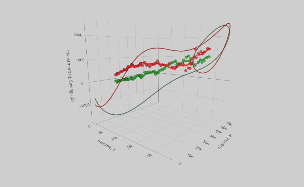
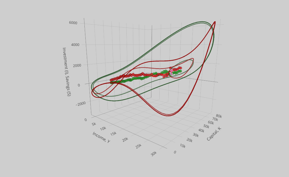
To visualize the mechanism of Kaldor’s model, we need to find a limit cycle. The reader that has gone this far will have no trouble to find one by changing just about any parameter in this (kind of wacky) model. Let’s just point out that, as remarked by Chang and Smyth, changes in the speed of adjustment can have dramatic results on the behavior of the model, without changing the phase diagram and the number of equilibria. Increasing the value of \(\alpha\) to 0.3 thus will give rise to a limit cycle of gigantic proportions (unfortunately, most limit cycles for those parameters bears those proportions that lead to a complete collapse of income below the zero level - but now that we have come so far, let’s not allow this to stop us from interpreting the cycle).
While the limit cycle is perhaps most clearly seen in the ‘Phase diagram’ and ‘Trajectories’ panels (increasing the “Final time” also helps), the 3d plot in the first panel gives us the most interesting way to illustrate Kaldor’s mechanism. After an initial increase much higher than with the lower speed of adjustment, both investment and saving show a sharp reversal, with savings consistently above investment for the whole way down to extremely low levels of income, capital, investment and savings. This corresponds to stage III of Kaldor’s model, when the savings curve is above the investment curve and the economy slides to the lower equilibrium (in the (gdp, savings / investment) plane of Kaldor’s figure 6).
At some point during this catastrophic fall, investment starts to go up again and eventually crosses above the level of savings at a very low level of income and capital. The economy can start its long path toward an even higher equilibrium than before.
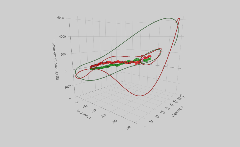
While savings are initially way below investment (or in other words, people are borrowing heavily and investment soars), it starts to soar when income has sufficiently increased and the rapid accumulation of capital slows down the increase of investment, until savings catches up and after overtaking investment, triggers a new collapse. After that, the cycle repeats in a rather pleasant looking loop, although not a very accurate one from a purely economic point of view. But the movement corresponds rather well to the mechanism described in 1940 by Kaldor.
Notes
-
Kaldor, Nicholas. 1940. “A Model of the Trade Cycle.” The Economic Journal 50(197):78–92. doi: 10.2307/2225740. url: http://www.jstor.org/stable/2225740 ↩
-
Chang, W. W., and D. J. Smyth. 1971. “The Existence and Persistence of Cycles in a Non-Linear Model: Kaldor’s 1940 Model Re-Examined.” The Review of Economic Studies 38(1):37–44. doi: 10.2307/2296620. url: http://www.jstor.org/stable/2296620. Another mathematical formalisation of Kaldor’s model can be found in Black, J. 1956. “A Note on Mr. Kaldor’s Trade Cycle Model.” Oxford Economic Papers 8(2):151–63. doi: 10.1093/oxfordjournals.oep.a042259. url: https://academic.oup.com/oep/article/8/2/151/2362202 ↩
-
Although my current work with Michaël Assous on the early macrodynamic models has shown that this was not always the case; in particular, Jan Tinbergen built several models that could explain both local, limited fluctuations maintained around an equilibrium point and the possibility of global instability and collapse either to a low equilibrium level or to a zero level in the most extreme cases. See in particular our WP “Jan Tinbergen’s early contribution to macrodynamics (1932-1936): multiple equilibria, complete collapse and the Great Depression” https://halshs.archives-ouvertes.fr/halshs-03087375 and a forthcoming book on the subject. ↩
-
The stability of those equilibria can easily be seen graphically: whenever savings is above investment, the activity will have a tendency to decrease to reestablish the equilibrium between them. On the contrary if investment is above saving, the activity will increase until savings are at the level of investment. Thus we see that going above and on the right of point C, the level of activity will have a tendency to increase to point B, etc. ↩
-
The data used to estimate the relationships between investment, savings, GDP and the stock of capital are taken from the Federal Reserve Bank of Saint Louis website. The series used are Personal Saving Rate, Real Gross Domestic Product, Net domestic investment and Capital Stock. ↩
-
This econometric approach is obviously not very rigorous and it should in no way be taken at face value but rather as an easy way to specify our functions’ shapes to explore numerically the perception of cycles contained in Kaldor’s article and Chang and Smyth’s article. The whole point of this blog is really to develop new computational tools and visualization to understand the history of economic thought and models and I hope the reader will excuse the casual treatment of econometric relationships. ↩
-
Klein, L. R., and R. S. Preston. 1969. “Stochastic Nonlinear Models.” Econometrica 37(1):95–106. doi: 10.2307/1909208. url: http://www.jstor.org/stable/1909208 ↩